← Back to Blog

This work reproduces results from an interesting paper Visual symbolic mechanisms: Emergent symbol processing in Vision Language Models (arxiv, openreview) published in ICLR 2026 (Oral). The reproduction code is available at GitHub. While most results can be successfully reproduced, others do not look good. So revisions and improvements are welcome.

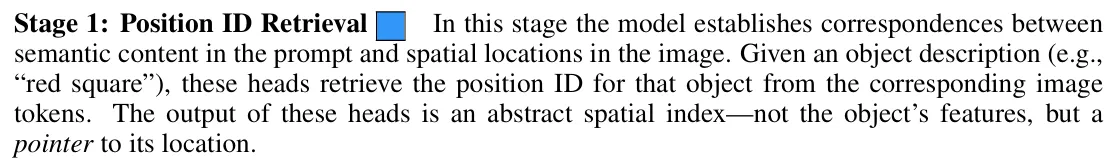
The Three-Stage Hypothesis

This paper proposes a three-stage hypothesis for the emergent symbolic binding mechanisms in Vision Language Models (VLMs). First, the ID retrieval heads retrieve the so-called position-IDs of the objects mentioned in the prompt from an image. Second, the ID selection heads figure out the position-ID of the missing object in the prompt (this object is called a “target object”). Third, the feature retrieval heads use the position ID retrieved in stage 2 to retrieve the features (color or shape) of the missing object.

For example, if a VLM takes as input an image containing a red square and a blue circle and a prompt saying In this image there is a red square and a, then the ID retrieval heads find the position ID of “red square”, the ID selection heads conclude the missing object is the other object in the image, and the feature retrieval heads retrieve the semantic features of the target object, i.e., blue and circle.

The position-ID can be understood as a pointer to the object’s location represented by the vectors stored somewhere in the heads (Section 3.2):

In this reproduction, we are using the input of the output projection of each head for stage 1 and 2 as the paper claims it’s analyzing the causal effect of the output of attention heads in Section 3.4 and the information from distinct heads will be blended during the output projection of the head.

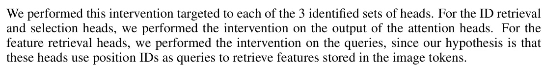
For stage 3, however, we are using the output of query or key projection of each head for different experiments as described in the paper. For example, in the intervention experiment with photorealistic images (Section 4.2), the authors describe it as follows,

And in the experiment for the localization of position IDs (Section 4.3), they state the following,

Therefore, we implement it in our reproduction like this,

if stage == 4:    # for section 4.3
    hs_input = target_layer.self_attn.k_proj.output[0]
elif stage == 3:    # Feature Retrieval
    hs_input = target_layer.self_attn.q_proj.output[0]
else:             # Intercept input to o_proj
    hs_input = target_layer.self_attn.o_proj.input[0]

Analysis Methods And Results

To prove their three-stage hypothesis, the paper uses three methods: principal component analysis (PCA), representational similarity analysis (RSA) and causal mediation analysis (CMA).

Principal Component Analysis (PCA)

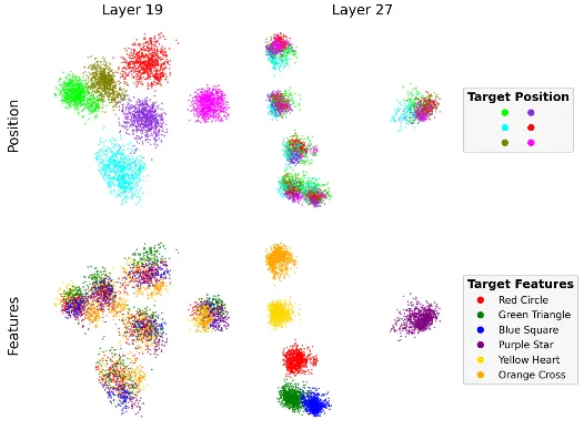
The principal components are an orthonormal basis that best fits the data. This paper extracts the first two principal components and plots the corresponding coefficients as the coordinates in a plane. In order to correctly output the missing object, the model needs to make different positions separable in stage 2 and different features distinguishable in stage 3. Figure 1(b) shows the result:

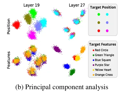
where it uses layers 19 and 27 as representatives of stages 2 and 3, respectively.

Our reproduction shows the same result:

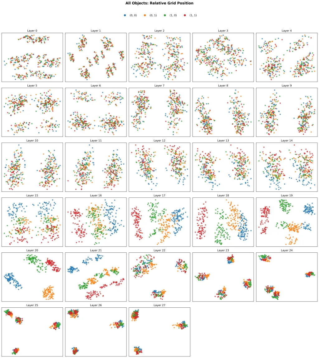
The authors also included a sweeping result across all layers for the analyses of relative vs. absolute spatial coding in their May update. For example, this is the PCA results colored by target object relative position for all objects (Appendix A.5.3):

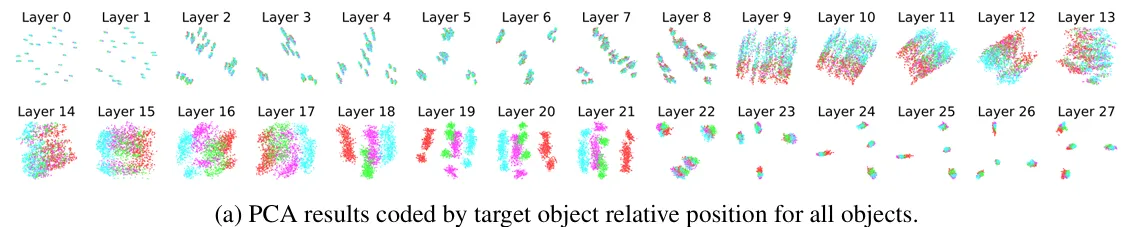
And our reproduction coincides with it:

Our reproduction has similar results for other PCA analyses, too (see details at link). Note that the caption of Figure 26(c) repeats that of Figure 26(e) in the May version, which we believe should instead be “PCA results colored by target object features for all objects.” based on the text describing the experiments. Nevertheless, the plot is similar to our reproduced result based on our understanding of the text.

In all other experiments we number the figures in accordance with the January version of the paper since we had run some experiments by the time the paper was updated in May.

Representational Similarity Analysis (RSA)

RSA is a method borrowed from the paper Representational Similarity Analysis – Connecting the Branches of Systems Neuroscience (link). In its original setting, a representational dissimilarity matrix (RDM) is used to relate representations in brains and models or activity patterns measured with different techniques. An RDM is computed as follows,

…For each pair of experimental conditions, the associated activity patterns (in a brain region or model) are compared by spatial correlation. The dissimilarity between them is measured as 1 minus the correlation (0 for perfect correlation, 1 for no correlation, 2 for perfect anticorrelation). These dissimilarities for all pairs of conditions are assembled in the RDM. Each cell of the RDM, thus, compares the response patterns elicited by two images. As a consequence, an RDM is symmetric about a diagonal of zeros…

After getting the RDMs, we are able to compute their correlation,

RDMs can be quantitatively compared just like activity patterns, e.g., using correlation distance (1-correlation) or rank-correlation distance. Because RDMs are symmetric about a diagonal of zeros, we will apply these measures using only the upper (or equivalently the lower) triangle of the matrices.

In the ICLR paper, the authors use representational similarity matrices (RSMs) instead (Section 3.3, Appendix A.2),

Their RSA results show that the three correlation peaks appear in the order that the three-stage hypothesis predicts across all models. Our reproduction indicates a similar conclusion with some minor discrepancies.

First, the correlation scores for the feature of the last token have a single peak at the last layers in the paper, but our result shows the curve has a bimodal distribution with one peak at the first layers and the other at the last layers.

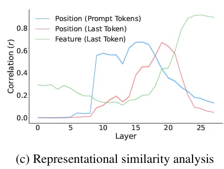Figure 1(c) (for Qwen2-VL) in the paper

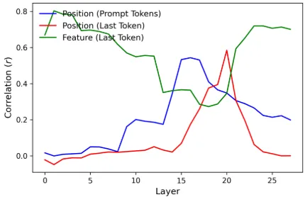Reproduced Figure 1(c) (for Qwen2-VL)

Second, our reproduction for LLaVA1.5-7b does not show as strong results as in the paper, especially for position of the last token (or target position).

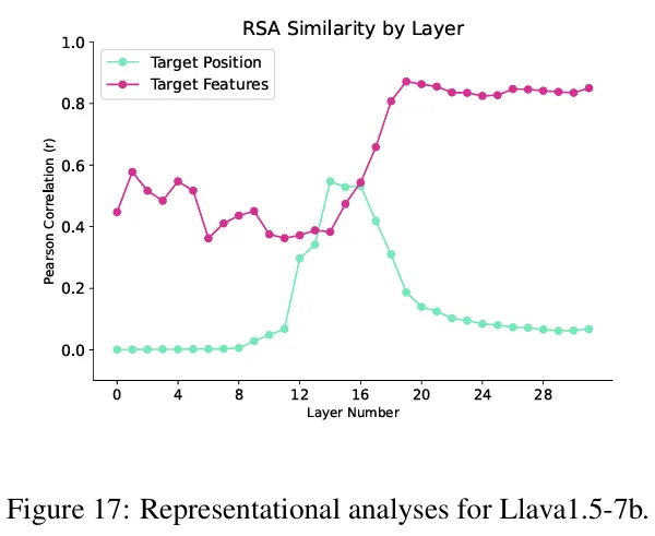Figure 17 (for LLaVA1.5-7b)

Reproduced Figure 17 (for LLaVA1.5-7b)

RSA is also used to determine whether position IDs are relative or absolute as well as the effect of feature entropy on position IDs. We reproduced these results with minor differences, too (details at link).

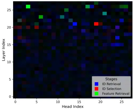
Causal Mediation Analysis (CMA)

CMA is used to identify which heads are responsible for which one of the three hypothesized stages. Details from the paper are shown below.

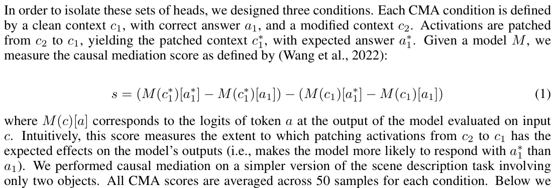
Due to limited budget, we only perform causal mediation on one sample for each condition, which may to some extent explain the discrepancies between our reproduction and the paper in subsequent experiments.

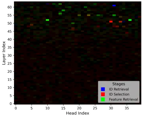
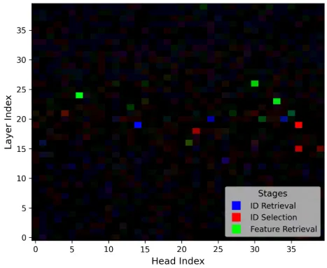
At first, the authors use CMA to find mediation scores over all heads and models. For instance, Figure 1(d) shows the CMA results for Qwen2-VL:

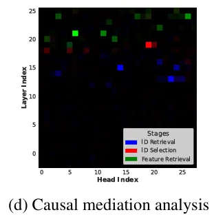
Our reproduction shows the same trend, though not exactly the same,

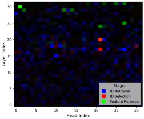
Most models we test show similar results to the paper, while models like Qwen-2.5-VL-32b, LLaVA-1.5-13b and LLaVA-OneVision have intertwined heads as shown below.

Reproduced CMA results for Qwen-2.5-VL-32b

Reproduced CMA results for LLaVA-1.5-13b

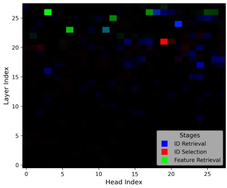Reproduced CMA results for LLaVA-OneVision

We additionally test Idefics2-8b, which shows the same trend of three stages:

On top of these CMA scores, the authors conduct various intervention experiments.

In the photorealistic intervention experiments (Section 4.2), the paper shows high intervention accuracies across all heads and models, while our reproduction does not show the same results for ID retrieval heads in LLaVA models:

Figure 3(b) in the paper

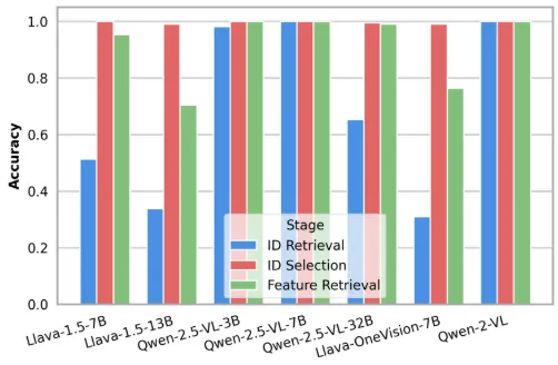Reproduced Figure 3(b)

In the experiment to show position IDs are localized in object patches (Section 4.3), it turns out the prompt from the paper does not work well because LLaVA models would think the sentence has been completed and just output an end-of-sequence token (</s>).

To make these models actually predict a color for testing, we use this prompt instead:

prompt = f"In this image what is the color of the {shape_list[i][pos]}. Answer with the correct color only. Answer:"

Despite this fix, we still cannot reproduce similar results as shown in the paper:

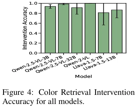Figure 4 in the paper

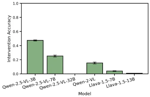Reproduced Figure 4

The reasons might include that the CMA scores from previous experiments are not generalizable enough and that the accuracy heavily depends on prompt design and implementation details like how to determine the tokens that span an object in the image.

In order to investigate whether the generalizability of CMA scores affects the accuracy, we updated our experiment with 36 samples for LLaVA-1.5-7b (see the update in commit), but it did not improve the accuracy (see the comparison in commit).

In the experiment for the reusability of position IDs (Section 4.4), we append Answer: to the prompt from the paper for the same reason and reproduce similar results with LLaVA models as exceptions again:

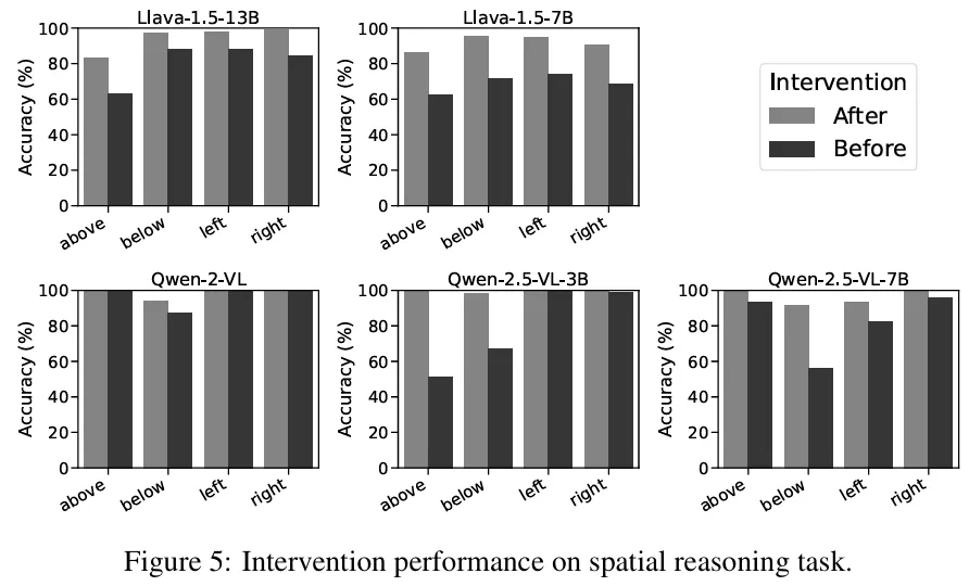Figure 5 in the paper

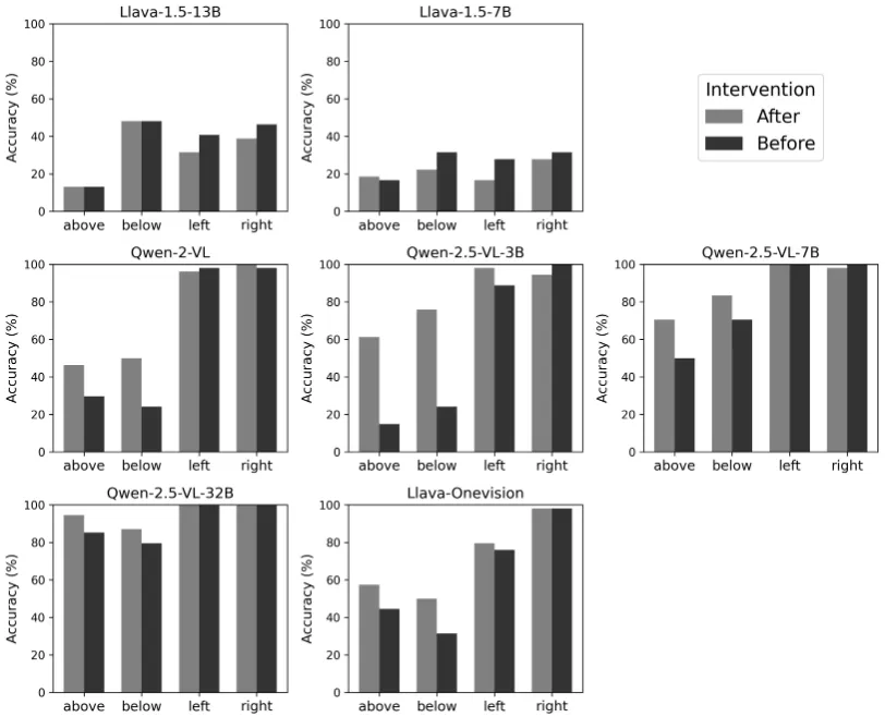Reproduced Figure 5. We additionally test Qwen2.5-32B and LLaVA-OneVision.

We are able to reproduce the intervention results for relative vs. absolute spatial encoding (Appendix A.5.3, Figure 29), while LLaVA models show less intervention accuracy in the experiment with the COCO dataset (Appendix B, Figure 45).

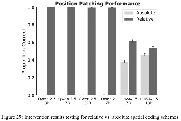Figure 29 in the paper

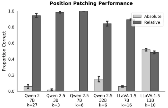Reproduced Figure 29. We run a sweeping on k over 0 to 99
and choose the best result for each model.

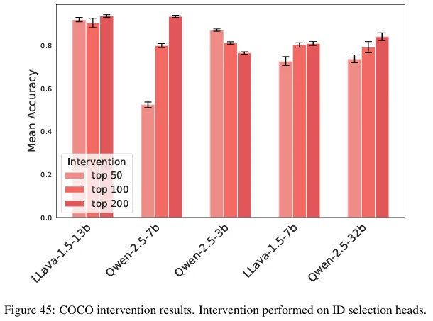Figure 45 in the paper

Reproduced Figure 45

In the counting experiment (Appendix C), our results show the accuracies are close between the ablations of the max and the bottom top k heads, while Figure 46 in the paper shows a maximum gap of >0.8 on the same condition. It might be attributed to ungeneralizable CMA scores and implementation details.

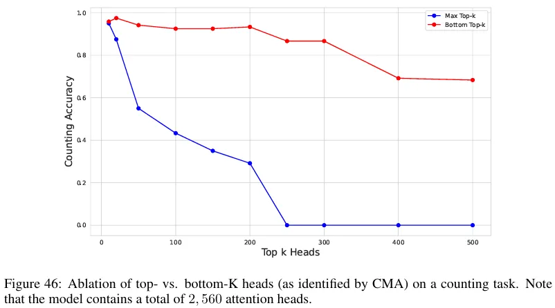Figure 46 in the paper

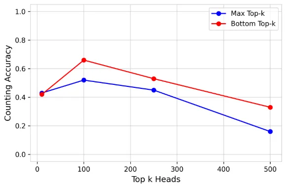Reproduced Figure 46

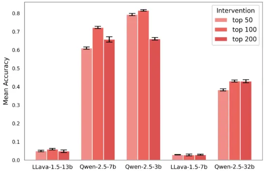
The last experiment is the intervention on low-entropy scene description tasks (Appendix D). Since the paper does not specify the k value they used in their experiment, we ran a sweeping experiment beforehand with fewer samples over a set of k values. The best k value found is k=50. While our reproduction shows this kind of intervention can improve the accuracy in the low-entropy condition, the improvement is not as much as that in the paper, mainly because the base accuracy has already been very high for Qwen models and images with a 2x2 grid.

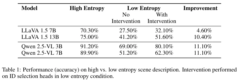Table 1 in the paper

Model	High Entropy	Low Entropy (No Intervention)	Low Entropy (With Intervention)	Improvement
LLaVA 1.5 7B	66.57%	44.54%	48.69%	4.15%
LLaVA 1.5 13B	76.32%	70.47%	78.15%	7.68%
Qwen 2.5-VL 3B	98.99%	92.89%	92.64%	-0.25%
Qwen 2.5-VL 7B	97.90%	95.53%	98.99%	3.46%
Qwen 2-VL 7B	99.83%	94.07%	91.14%	-2.94%

Reproduced Table 1 for images with 3x3 grid. Note that we additionally test Qwen 2-VL 7B.

Model	High Entropy	Low Entropy (No Intervention)	Low Entropy (With Intervention)	Improvement
LLaVA 1.5 7B	100.00%	98.96%	98.96%	0.00%
LLaVA 1.5 13B	98.96%	98.96%	100.00%	1.04%
Qwen 2.5-VL 3B	100.00%	100.00%	100.00%	0.00%
Qwen 2.5-VL 7B	100.00%	100.00%	100.00%	0.00%
Qwen 2-VL 7B	100.00%	100.00%	100.00%	0.00%

Reproduced Table 1 for images with 2x2 grid.

Acknowledgements

Anyone who makes contributions or helps improve this reproduction, especially for Figure 4, Figure 46 and the results on LLaVA models, will appear here.

← Back to Blog